Process Synchronization-Part 3 (Flag Array Solution)

Till now, we have discussed the following posts on Process Synchronization. Before reading this post, please read the following post on Process Synchronization:-

• Part 1: The Critical Section Problem
• Part 2: Turn Variable Solution

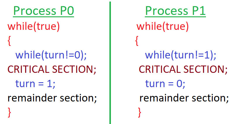
In the previous post, we discussed a solution to the 2-process synchronization problem which did not satisfy PROGRESS. Let us examine why the problem arose.

In the solution above, no process is being made to state explicitly that it is interested to enter its critical section. An inherent assumption is being made that both the processes will always be interested to enter their critical section but this might not be the case. In our next solution, we try to rectify this problem using a 2-element boolean flag array.

• flag[0] = 1 means Process P0 is interested to enter its critical section
• flag[0] = 0 means Process P0 is not interested to enter its critical section
• flag[1] = 1 means Process P1 is interested to enter its critical section
• flag[1] = 0 means Process P1 is not interested to enter its critical section

Analysis

• Before attempting to enter its critical section, each process sets its flag variable to true indicating that it is interested to enter its critical section.
• Each process than waits in a loop until the other process has its flag value to false. This means that a process will wait in the loop as long as the other process has set its flag value to true and has not yet set it to false, meaning that the other process is currently holding the pass to enter critical section.
• Let us say Process P1 has set its flag value to true which means it has executed the statement flag[1] = true;
• Now, it gets pre-empted and Process P0 enters the scene and sets flag[0] = true;
• Process P0 will then enter the waiting loop until Process P1 comes back, enters critical section, exits and sets flag[1] = false;
• So, in this solution, the process which sets its flag value to true earlier will get to enter its critical section earlier.

Mutual Exclusion

Suppose Process P0 is currently inside its critical section. This means it has set flag[0] to true. If Process P1 now attempts to enter its critical section, it will wait in the loop because flag[0] will be true as long as P0 is inside its critical section. So, mutual exclusion HOLDS.

Progress

We need to analyze a few things here.

• Let P0 be interested to enter its critical section while P1 is not yet in the scene.
• P0 sets flag[0] = true;
• while(flag[1]==true) is false so it exits waiting loop and enters critical section.
• P0 sets flag[0] to false;
• Now, let us say P0 wants to enter its critical section once again.
• P0 sets flag[0] = true;
• while(flag[1]==true) is false so it exits waiting loop and enters critical section.
• P0 sets flag[0] to false;

So, a non-interested process P1 has not blocked an interested process P0 from entering its critical section.

**Whenever I use the term 'enter its critical section', it means that a particular process is entering its own critical section. Note that a process can enter only its own critical section. A critical section of a process is a code segment of the process which accesses shared variables. A process is a program in execution. A program consists of lines of code. Ok! Enough :P

So, for now, we can think that this solution satisfies progress. But we must analyze another situation before concluding the same.

• Let P0 be interested to enter its critical section while P1 is not yet in the scene.
• P0 sets flag[0] = true;
• At this point somehow P0 gets pre-empted, P1 enters the scene and executes flag[1] = true;
• So, now, flag[0] and flag[1] are both true;
• Now, if P0 comes back and starts executing from where it left off, which means from the while(flag[1]==true); statement, it finds that flag[1] is true and it has to wait. If P0 gets pre-empted and P1 comes, P1 has to wait as well as flag[0] is also true. So, we have a DEADLOCK situation and so, PROGRESS is not satisfied by this solution.

Bounded Waiting

We know that the definition of bounded waiting says that there should be a finite bound on the number of times other processes are allowed to enter their critical sections after the said process has exhibited its interest to join the critical section and before it is granted the chance. Here, each process exhibits its interest by setting its flag to true. And, this should hold for all processes.

Let us suppose P1 has set its flag to true and has then pre-empted. Now, if P0 comes, executes its critical section, and exits after setting flag[0] to true, instantly P1 can be granted the chance as it can now come out of the waiting loop. So, bounded waiting HOLDS.

Conclusion

So, even now, we do not have a correct solution to the 2-process synchronization problem. In the next post, we will look at Peterson's Solution which makes a small modification to the algorithm described in this post, to provide a correct solution.

Was it a nice read? Please subscribe to the blog by clicking on the 'Follow' button on the right hand side of this page. You can also subscribe by email by entering your email id in the box provided. In that case, you will be updated via email as and when new posts are published.Also, please like the Facebook Page for this blog at Gate Computer Science Ideas. Cheers!

Click here to read Part 4

Process Synchronization-Part 2 (Turn Variable Solution)

Till now, we have covered the Introduction to Process Synchronization up to the Critical Section Problem. Before reading this post, please read the following post on Process Synchronization:-

• Part 1: The Critical Section Problem

In this post, we will see the 1st solution to the 2-process synchronization problem which uses a shared variable turn. We name the 2 processes P0 and P1.

Turn Variable Solution to 2-process Synchronization Problem

The solution code can be shown by the diagram below:-

Analysis

• turn is a shared boolean variable which can hold the value either 0 or 1
• Process P0 waits in an infinite loop until turn value is 0, only then can it enter the Critical Section
• When P0 exits Critical Section, it sets turn = 1 to enable Process P1 to enter the Critical Section
• The code is extremely symmetric and easy to understand. Please observe it with some time in hand.

We will now analyze the Turn Variable algorithm with respect to the 3 conditions in our previous post.

Mutual Exclusion

Let Process P0 be in its critical section. This means that turn = 0 at the moment. Until and unless P0 exits critical section and sets turn = 1, Process P1 cannot enter the critical section. The analysis is similar if we start with process P1. So, mutual exclusion HOLDS.

Progress

Let Process P0 be inside its critical section. It finishes its critical section and sets turn = 1. Now, let us assume P0 again wants to enter its critical section. It will not be able to, as long as Process P1 enters its critical section at least once and sets turn = 0 after exiting. So, if Process P1 is not interested to enter its critical section, in a way, it is blocking the entry of an interested process P0 to the critical section even though there is no process currently in its critical section. So, Progress DOES NOT HOLD.

BOUNDED WAITING

Here, we find that strict alternation exists. In other words, the only possible execution sequence is one process followed by the other. So, bounded waiting definitely HOLDS.

Conclusion

This is an incorrect solution to the 2-process synchronization problem as Progress does not hold. In the next post, we will analyze the exact reason why this problem is occurring and try to develop a better solution.

      Was it a nice read? Please subscribe to the blog by clicking on the 'Follow' button on the right hand side of this page. You can also subscribe by email by entering your email id in the box provided. In that case, you will be updated via email as and when new posts are published.Also, please like the Facebook Page for this blog at Gate Computer Science Ideas. Cheers!



Click here to read Part 3

Process Synchronization- Part 1 (The Critical Section Problem)

This topic is extremely important for GATE. Also, most of us find it confusing. In this series, we will try to cover the basic essentials required to solve GATE questions (trust me, not much depth in this topic is needed for GATE!). The topics will include the following:-

• Race Condition and The Critical Section Problem
• Solutions to the 2-process Synchronization Problem
• Hardware solutions including the Test, Set and Lock (TSL)
• Semaphores, Mutexes and the difference between them
• Applications of Semaphores
• A couple of classic synchronization problems 
• Very important previous GATE questions

Race Condition

Most of us are familiar with the notion of a process. A process can be thought of as a program in execution. In a uni-processing environment, only 1 process can be running at a time. Suppose there are 10 processes to be executed on a certain computer. Process 1 starts executing and in the midst of its execution, it requires some I/O time. So, during this time, if we keep the CPU idle, it will be a wastage and we will obtain reduced throughput. What we can do is, some other process can execute on CPU in the mean time. In this way, the CPU is always kept busy (that is the aim).

But this constant getting-in and throwing-out of processes from the CPU comes with a price. When there are so many processes executing with an effective idea of togetherness, consistency can be hard to achieve, especially when there are shared variables involved. Also, depending on order of execution of processes, the results obtained may be different. We will examine all these ideas.

Let us consider the famous Producer-Consumer problem to understand what a race condition is. While we do not need to analyze the exact code for this problem, we must understand intuitively what the problem is. In the Producer-Consumer problem, there are 2 processes, a Producer process and a Consumer process. Also, we have an array/buffer of items, let us consider the array to be infinite for now. 

To maintain the number of items available in the buffer/array, a shared variable count is needed. It is a shared variable because both the processes should be able to modify it. When the Producer process produces an item and places it on the buffer, it should increment by 1 (execute the statement count++). When the Consumer process takes up an item from the buffer, it should decrement count by 1 (execute the statement count--).

But count++ and count-- are not atomic statements at the Assembly Language Level. In other words, these statements are individually executed as a series of 3 atomic statements shown below:-

Let initial value of count be 18. We have numbered the statements from 1 to 6 for ease of analysis. Note that atomic statements can be individually in any order, which means that after execution of statement 1, the Producer process may be pre-empted while the Consumer process executes statement 4. So, (1,2,3,4,5,6) is a possible execution sequence. Also, (1,4,2,5,3,6) is another possible execution sequence.

When the sequence (1,2,3,4,5,6) occurs, the following happens:-

• reg1 = 18
• reg1 = 18+1 = 19
• count = 19
• reg2 = 19
• reg2 = 19-1 =18
• count = 18           (final value of count is 18-->correct)

So we find that the desired result is obtained. Now, let us see what happens when the sequence (1,2,4,5,3,6) occurs:-

• reg1 = 18
• reg2 = 18
• reg1 = 18+1 = 19
• reg2 = 18-1 = 17
• count = reg1 = 19
• count = reg2 = 17  (final value of count is 17--> incorrect)

If we interchange the final 2 statements in the above sequence so that (1,2,4,5,6,3) occurs, the following happens:-

• reg1 = 18
• reg2 = 18
• reg1 = 18+1 = 19
• reg2 = 18-1 = 17
• count = reg2 = 17
• count = reg1 = 19       (final value of count is 17--> incorrect)

So, in both the above cases, the final value of count is inconsistent and undesired. Depending on which process executes last, the final value of count is changing. This is called a race condition.

Race condition is a situation where several processes access and manipulate shared data concurrently. The final value of the shared data depends on the process which finishes last. Concurrent processes must be synchronized to prevent race conditions.

The Critical Section Problem

Suppose there are n processes, each having a particular section of code where it accesses shared variables. So, each process has a code segment where it accesses shared data which is called the critical section. We must ensure that when 1 process is executing in its critical section, no other process must be allowed to execute in its critical section.

The general code structure of process i can be shown by the diagram below:-

The entry section is usually used to obtain locks on shared variables and permission to access the Critical Section. 

The exit section is usually used to release locks on shared variables so that other processes can access their critical sections.

The remainder section is a code segment not related to the critical section.

The code is shown in a do-while loop with the assumption that a process will end when it executes some code in its remainder section which causes it to terminate.

Critical Section Problem Solution Requirements

Any solution to a critical section problem must satisfy the following 2 conditions mandatorily:-

• Mutual Exclusion: When a process i is executing in its critical section, no other process should be allowed to enter its critical section.
  
• Progress: If no process is in its critical section and we have some process which is interested to enter its critical section, only those processes not in their remainder section should be allowed to participate in the decision of which process will get the chance to enter the critical section next. In other words, only those processes which are interested to enter the critical section should be able to influence which process gets the chance to enter the critical section. A non-interested process should not be able to block an interested process from entering the critical section.

**Note: If there is INFINITE WAITING TIME TO MAKE ABOVE DECISION (which also includes the notion of DEADLOCK)  to make above decision, that means there is NO PROGRESS. This particular point is very important for GATE.

A solution to the critical section problem should ideally satisfy another condition known as Bounded Waiting the definition of which is not the same across textbooks. We can think of bounded waiting as the assurance implicit to the process that there will be a bound (finite upper limit even if it is a very high number) on the number of times other processes are allowed to enter the critical section after that process has requested to enter the critical section and before that request is granted.

In this post, we have seen up to the Critical Section Problem. In the next post, we will see various solutions to the 2-process Synchronization problem where we have only 2 processes.

Click here to read Part 2

Was it a nice read? Please subscribe to the blog by clicking on the 'Follow' button on the right hand side of this page. You can also subscribe by email by entering your email id in the box provided. In that case, you will be updated via email as and when new posts are published.Also, please like the Facebook Page for this blog at Gate Computer Science Ideas. Cheers!

Database Normalization--Part 4 (Normal Forms)

Till now, we have covered up to the types of functional dependencies. Before reading this post, please read the following posts on Normalization:-

• Part 1: Introduction to Database Normalization
• Part 2: Closure Set of Attributes Method
• Part 3: Types of Functional Dependencies

In this post, we look at some important definitions and move up to the hierarchy of normal forms. Also, we show how to state the highest normal form of a relation. 

**This post is entirely theory and may be boring. It requires multiple readings.

Prime Attribute

·         Any attribute which is part of at least one candidate key is called a prime attribute.

·         If AF is a candidate key, then A and F are prime attributes.

Non-prime attribute

·         An attribute in a relation which is not part of any candidate key is called a non-prime attribute.

·         If in a relation R(A,B,C,D,E) , AD is the only candidate key, then B,C and E are non-prime attributes.

Normal Forms

·         It is a property of relations which indicates the amount of redundancy in the relation.

·         Normal form and degree of redundancy are inversely proportional.

·         Normalization is a systematic approach applied on relations to reduce the degree of redundancy and achieve progressively higher normal forms.

Normalization Procedure

1)      Determine the highest possible normal form of the given relation.

2)      Decompose the relation from its existing normal form to higher normal forms.

Procedure to find highest Normal Form of the given relation

1)      Find all possible Candidate Keys of the given relation.

2)      Identify all the existing prime and non-prime attributes.

3)      Identify all the existing Full Dependencies, Partial Dependencies, Transitive Dependencies and Overlapping Candidate Key Dependencies.

4)      Refer to the definition and hierarchy of Normal Forms for finding the highest possible Normal Form of the given relation.

Hierarchy of Normal Forms

Normalization is a hierarchical procedure and each stage is designated by a particular normal form. The hierarchy of normal forms has been shown in the diagram given below:-

First Normal Form (1NF)

·         A relation is said to be in 1NF if all the values in the relation are atomic and single-valued.

·         According to Codd’s rules of Relational Database Management Systems, every relation will always be in 1NF by default.

·         The relation instance given below does not satisfy 1NF criterion (it is not in 1NF) as Email is not a single-valued attribute.

Name	Class	Email
Ravi	1	ravi@gmail.com ravi@yahoo.com
Rahul	2	rahul@gmail.com
Rakesh	4	rakesh@hotmail.com

·         The above relation instance can be converted to 1NF as shown below:-

Name	Class	Email
Ravi	1	ravi@gmail.com
Ravi	1	ravi@yahoo.com
Rahul	2	rahul@gmail.com
Rakesh	4	rakesh@hotmail.com

Second Normal Form (2NF)

A relation is said to be in 2NF if:-

·         It is in 1NF.

·         It has no partial dependencies.

Third Normal Form (3NF)

A relation is said to be in 3NF if:-

·         it is in 2NF.

·         It has no transitive dependencies.

Boyce Codd Normal Form (BCNF)

A relation is said to be in BCNF if:-

·         it is in 3NF and has no overlapping candidate key dependencies.

The hierarchy of Normal Forms can be represented by the above diagram. So, if a relation is in BCNF, it has to be in 3NF already but the reverse may not be true. Similar statments can be made for the other normal forms as well.

In this post, we have seen the hierarchy of Normal Forms. In the next post, we will look at examples on Normal Forms.

Was it a nice read? Please subscribe to the blog by clicking on the 'Follow' button on the right hand side of this page. You can also subscribe by email by entering your email id in the box provided. In that case, you will be updated via email as and when new posts are published. Cheers!

Click here to read Part 5

Database Normalization--Part 3 (Types of Functional Dependencies)

Till now, we have covered up to the Closure Set of Attributes method of finding candidate keys. Before reading this post, please read the following posts on Normalization:-

• Part 1: Introduction to Database Normalization
• Part 2: Closure Set of Attributes Method

In this post, we will look at the types of Functional Dependencies which is very important for understanding Database Normalization. Here, we look at 4 types of Functional Dependencies:-

• Full Dependencies
• Partial Dependencies
• Transitive Dependencies
• Overlapping Candidate Key Dependencies

****For GATE, it is very important to know and remember the exact criterion of each of these dependencies. Almost every year, at least 1 direct question comes from this topic.

Full Dependencies

·       A dependency is said to be full if the determinant of the dependency is a superkey.

·         Full dependencies can be represented by the diagram shown above:-

The amount of redundancy caused by each full dependency is always 0, hence normalization procedure will not try eliminating Full Dependencies. An example of a full dependency has also been shown above. The candidate key has been assumed.Partial Dependencies

·         A dependency is said to be partial if non-prime attributes are depending partially on a candidate key. In other words, if there is a functional dependency in which part of a candidate key is determining non prime attribute(s), then it is called a partial dependency.

·       Partial dependencies can cause redundancy in the relations and hence they will be eliminated in the normalization procedure.

·       If there exists a relation that has simple candidate keys only(single attribute candidate keys), then there exists no partial dependencies.

·         Partial dependencies can be represented by the diagram shown above. An example for the same has also been shown.

Transitive Dependencies

·         A dependency is said to be transitive if a non-prime attribute(s) are depending on other non-prime attributes or on a combination of non-prime attributes and proper subject of candidate keys. In other words, the dependency is transitive if one or more non-prime attributes are depending on a superkey transitively but not directly.

·         Transitive dependencies can cause redundancy hence normalization process tries to eliminate them.

·         If all attributes in a relation are prime, the number of partial dependencies and the number of transitive dependencies are both zero. (Why? Think!)

·      Transitive dependencies can be represented by the diagram shown above. An example for the same has also been shown.

Overlapping Candidate Key Dependencies

·         If in a dependency XàY, X is not a superkey and Y is the proper subset of a candidate key, then the dependency is called an Overlapping Candidate Key dependency.

·         Overlapping Candidate Key Dependencies can be represented by the diagram shown above. An example for the same has also been shown.

In this post, we have seen the types of Functional Dependencies. In the next post, we will look at a few definitions and develop the concept of Normal Forms.

Was it a nice read? Please subscribe to the blog by clicking on the 'Follow' button on the right hand side of this page. You can also subscribe by email by entering your email id in the box provided. In that case, you will be updated via email as and when new posts are published. Cheers!

Click here to read Part 4

Database Normalization--Part 2 (Closure Set of Attributes)

Till now, we have covered up to the Closure Set of Attributes method of finding candidate keys. Before reading this post, please read the following post on Normalization:-

• Part 1: Introduction to Database Normalization

In this post, we will see how to find the candidate keys of a relation using the Closure Set of Attributes Method. We must note that candidate keys can also be found out using the axioms of Functional Dependencies mentioned. But during the GATE examination, an attempt to save time is a must.

Closure Set of Attributes Method

This method is very useful in finding out the keys of a relation which is needed for Normalization procedure. Let us go through a couple of examples to understand the procedure.

Suppose we consider the following relation R with 4 attributes (A,B,C,D) and are also given a functional dependency set (Functional dependencies are arrived at during the Requirements Analysis Phase, when the problem is being analyzed and client specifications are being noted).

R(A,B,C,D) = { AàB , BàC , CàD , DàA } -----------> given FD set

So, here we have 4 functional dependencies. Now, we will find out the entire attribute set which each attribute derives. It is a repetitive approach.

(A)⁺ = { A,B,C,D}

Closure set of A contains A by default as AàA always holds. 
As we have the functional dependency AàB, so the closure set of A will contain B (A derives B)

Closure set of A contains B and B->C therefore using transitivity axiom,  we can say that AàC, so   the closure set of A will contain C. 
 Similarly, we arrive at the following conclusions:-

·         (B)⁺={A,B,C,D}

·         (C)⁺={A,B,C,D}

·         (D)⁺={A,B,C,D}

In this example, we find that each of the attributes A,B,C and D are the candidate keys as each of them individually derives all the attributes of this relation. A candidate key is a minimal superkey. There cannot exist any other candidate key for this relation because any superset (other than itself) of a candidate key is a superkey but not a candidate key. Please read the previous sentence again if you find the language confusing. Let us take another example.

Let us consider another relation R(A,B,C,D,E,F,G,H) along with its functional dependency set as
{ABàCD,DàE,EàF,BàA,FàG,GàH}. 

We are required to find out the Candidate Keys for this

relation R.

In the 1st step, we find the closure sets of the single attributes A,B,C and D to obtain:-

·         (A)⁺={A}

·         (B)⁺={A,B,C,D,E,F,G,H}

·         (C)⁺={C}

·         (D)⁺={D,E,F,G,H}

Now, at the conclusion of this 1st step, we are sure that B is a candidate key as it derives all the attributes. Also, we can conclude at this point that if any other candidate key exists for this relation, it will not have B in it (as any superset of a candidate key is a superkey but not a candidate key).

      Now, we must find the closure sets of AC, CD, AD (2-attribute closures). We note here that

(AC)⁺ denotes the set that A and C can derive together, repetitively. Here,

(AC)⁺ ={A,C}
(AD)⁺={A,D,E,F,G,H}
(CD)⁺={C,D,E,F,G,H}

So none of the 2-attribute sets are candidate keys. But we still should check for the 3-attribute set
ACD. Note that B shouldn't be part of this check as it itself is a candidate key and cannot be part

of any superset of itself.

(ACD)⁺={A,C,D,E,F,G,H}

So, ACD is not a candidate key as well as it cannot derive the attribute B.

Important Note

If we look carefully at the Functional Dependencies, we will find that B is not present in Right Hand Side of any of the Functional Dependencies. This indicates that B should be a part of any candidate key (otherwise B won't be derived).

Now, if B is a part of any candidate key of this relation, there cannot be any other candidate key as B is a single attribute candidate key. So, we could have directly stated that B is the only candidate key for this relation which would have saved a lot of time. This trick comes in very handy in GATE. Any attrribute which is not present in Right Hand Side of any of the Functional Dependencies of a given relation, has to be part of any candidate key of that relation.

At this point, we know how to find the candidate keys of any given relation provided we know the Functional Dependencies which exist for that relation. In the next post, we will look at the types of functional Dependencies that exist and subsequently move on to Normal Forms. 

Was it a nice read? Please subscribe to the blog by clicking on the 'Follow' button on the right hand side of this page. You can also subscribe by email by entering your email id in the box provided. In that case, you will be updated via email as and when new posts are published. Please share the post if you find it useful. Cheers!

Click here to read Part 3

Database Normalization--Part 1

This is the first post on this blog. It starts the topic of Database Normalization. We will be introducing the motivation behind normalization. Subsequent posts will extend the topic and conclude with important GATE questions.

Let us consider the following relational database instance:-

*This particular relation was used as an example by the teacher who taught me this subject and I think it is very nice :P

stid	stname	course	duration	fees
100	X	Java	60	10000
200	Y	Java	60	10000
300	Z	Java	60	10000

Here, we find that the rightmost three attributes have repetitive data. If we analyse further, we find that for a particular course , for example, Java, its duration and fees are fixed at a particular instance of time. So, it is meaningless to represent the duration and fees’ information with every tuple. 

A better approach would have been to just store course information with every tuple and maintain a separate relation (table) for storing information about courses. In this approach, 2 relations are used instead of 1 as shown in the diagrams above. That way, there is a significant conservation of storage space. Here, we find that a Redundancy has occurred. Database Normalization takes care of redundancies.

Database Normalization is the process of splitting relations into smaller relations with the purpose of eliminating redundancies.

Redundancies

In the previous example, we saw the redundancies. It is important to analyze what causes redundancies before moving on to its harmful effects. Redundancies are nothing but repetitions caused due to what are known as Functional Dependencies. In the previous example, the following two functional dependencies exist:- 

course --> duration
course --> fees

Malicious effects of Redundancies

Redundancies cause various harmful effects as follows:-

Wastage of Memory

We have already seen this in the above example.

Anomalies (Insertion, Deletion, Updation)

Let us consider updation anomalies. Suppose the fees for the Java course has increased to Rs. 12,000.

If we don't use normalization, we will have to update the new fees in all of the tuples which have Java as course. If by chance we miss at least 1 tuple, there will be an anomaly (a mistake). This is called an updation anomaly.

To prevent these problems from occurring, we go for database normalization.

Functional Dependencies

·        A functional dependency is of the form XàY where X is called the determinant of the functional dependency and Y is called the dependent of the functional dependency.

If the value of determinant attribute(s) gets duplicated in the relation, then the value of dependent attribute(s) also shall get duplicated accordingly.

·         If the value of the determinant attribute(s) is unique, the dependent attribute(s) can have any value (there is no restriction on the values that can be taken by the dependent attribute(s) in that case). This particular point is very important and there have been previous GATE questions asked exclusively on this point which we will see later

Let us consider the relation instance shown below:-

Animal	Height_in_feet
Cat	30
Dog	40
Cat	30
Human	2
Cat	30

The functional dependency Animalà Height_in_feet is sure to be valid for this relation instance as whenever the Animal attribute has been repeated, the corresponding value for the Height_in_feet attribute is also same. (Please note that these values are extremely ficticious :P ). We cannot say if this Functional Dependency is valid for the entire relation as only a part of it has been shown.

But if the height value in the coloured tuple were to be changed to be 31, we could have clearly stated that this functional dependency does not hold for this relation.

Trivial dependencies

A functional dependency Xà Y is said to be a trivial dependency iff X is a superkey of Y.

Axioms of Functional Dependencies

·         Reflexivity: Trivial dependencies always hold.

·         Augmentation: If X,Y and Z are sets of attributes and XàY holds, then XZàYZ also holds.

·         Transitivity: If X,Y and Z are sets of attributes and XàY and YàZ hold, then XàZ also holds.

The above three rules are known as Armstrong’s axioms. Using these, we can derive some secondary rules as given below:-

·         Decomposition: If XàYZ holds, then XàY and XàZ both hold individually.

·         Composition: If XàY and AàB hold, then XAàYB holds.

·         Union: If XàY and XàZ hold, then XàYZ holds.

In the next part, we will see how to find key attributes and continue with the types of functional dependencies and beyond. Was it a nice read? Cheers!

Click here to read Part 2